Premise

The objective we start with simple. I have a device which can get me a random number, hopefully uniformly distributed. Now using this device, I’m to generate other distributions.

I’ve most likely come across fragments of code which does this, without being able to generalize. I can recollect sometime back, when Harish told me something about taking a cumulative distribution function (CDF) and projecting on the y-axis, but it never really sunk in.

When I took Topics in Machine Learning in my undergrad final year, EXP3 algorithm in a Multi-Arm Bandit setting required me to draw an arm with the probabilities of the arms being updated at every step. I figured Jeremy Kun’s code segment was enough under the time constraints - and forgot about it in a while.

Around the start of this month, when I got to using temperature for adjusting a distribution to generate more likely but still diverse samples for a version of Karpathy’s char-rnn, I stumbled across sampling again, and that was it.

At this point, I strongly suspect Histogram Equalization which was taught in Digital Image Processing, which I implemented once and left to rust since then is also somehow connected to this.

This post is hence a visit down memory lane, linking and strengthening concepts I most likely missed in the past.

Let’s sample

I’ll be using pytorch for operating on tensors.

import torch.nn.functional as F
import torch
from matplotlib import pyplot as plt
%matplotlib inline

For our purposes, we use randn to generate a 1-D tensor of random numbers, on which we apply softmax to convert them to probabilities. These are the probabilites which we’ll use to sample indices.

n = 10
acts = torch.randn(n)
print(acts)
probs = F.softmax(acts, dim=0)

The following auxilliary function helps us visualize the distribution.

def plot_probs_bar(vals):
    H, = vals.size()
    xs = list(range(H))
    vals = vals/vals.sum()
    ys = vals.tolist()
    plt.ylim(0, 1)
    plt.bar(xs, ys)

plot_probs_bar(probs)

Inverse Transform Sampling

From wikipedia:

Let \(X\) be a random variable whose distribution can be described by the cumulative distribution \(F_{X}\). We want to generate values of which \(X\) are distributed according to this distribution.

The inverse transform sampling method works as follows:

1. Generate a random number \(u\) from the standard uniform distribution in the interval \([0,1]\).
   
2. Compute the value \(x\) such that \(F_X(x)=u\).
   
3. Take \(x\) to be the random number drawn from the distribution described by \(F_x\)

Step 2 is a whole lot easier if one can find \(F^{-1}\).

Python’s random.random() samples from a uniform distribution between \([0, 1)\). I guess that’ll suffice as a starting point. Let’s say we have to randomly choose one from n samples, each with probability given by probs[i], the following function can do the job.

Jeremy Kun’s draw is very similar.¹

import random

def draw(probs):
    val = random.random()
    csum = 0
    for i, p in enumerate(probs):
        csum  += p
        if csum > val:
            return i

Verification

How do we verify, in the limit of a lot of samples - if the distribution of selections look like what we intended? We simulate the situation, obviously. I make 10,000 draws to check if the counts when normalized looks like the probability distribution.

from collections import defaultdict

def check_sampling(probs):
    max_samples = 10000
    counter = defaultdict(int)
    for i in range(max_samples):
        choice = draw(probs)
        counter[choice] += 1

    vals = torch.Tensor(list(counter.values()))
    return plot_probs_bar(vals)

check_sampling(probs)

If the above plot ends up being similar to the one given by just probabilities, it works. Turns out, it works.

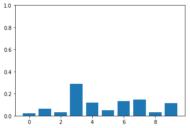
used for sampling

obtained after sampling

Karpathy’s Char RNN

The output layer of Karpathy’s char-rnn predicts probability of certain given classes. For a task like translation or nearly anything involving classification, argmax of the probabilities is the obvious choice. But since we’re hallucinating valid sequences - we have to randomly sample from the most probable choices.

For this, we skew the distribution to increase the probabilities of likely samples, and decreasing the probabilties of unlikely samples. Temperature acts as the control knob here, and the following illustration (hopefully) convinces why.

Temperature

\[ \mathrm{softmax}(x, T) = \frac{e^{x_i/T}}{\sum{e^{x_i/T}}}\]

I’ll model my TSoftmax as a functor, which uses pytorch’s nn.Module.

class TSoftmax(nn.Module):
    def __init__(self, temperature):
        super().__init__()
        self.T = temperature

    def forward(self, tensor):
        # Take all samples, divide them by T, pass through exp(x)
        entries = tensor.data.view(-1).div(self.T).exp()
        return entries/entries.sum()

If \(T = 1\), the above reduces to simple softmax. So, let’s try a few samples \(T \lt 1\), and \(T \gt 1\), see how the probability distribution we use to sample from changes.

m = 4
less_than_one = [2**(-b) for b in range(1, m)]
greater_than_one = [2**(b) for b in range(1, m)]

tvals = list(reversed(less_than_one)) + [1]  + greater_than_one
n_tvals = len(tvals)

plt.figure(figsize=(10, 30))

for i, T in enumerate(tvals):
    v = i+1
    ax1 = plt.subplot(n_tvals,1,v)
    ax1.set_title("t = {}".format(T))
    transform = TSoftmax(temperature = T)
    tprobs = transform(acts)
    plot_probs_bar(tprobs)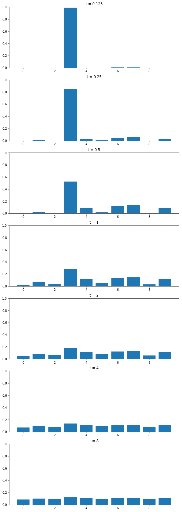

temperature variation

Increase in \(T\rightarrow \infty\) leads to uniform distribution, decrease in \(T \rightarrow 0\) leads to argmax situation. Thus, our good values for hallucinating could be somewhere in \([0.5, 0.7]\).